
Research on operation strategy of multiple channels pharmaceutical supply chain based on blockchain technology

Based on the problem description and decision assumptions outlined in the previous section, this section first discusses the reselling model (RN) and the agency selling model (SN) in the absence of blockchain technology. Subsequently, the paper explores the reselling model (RB) and agency selling model (SB) with blockchain technology, deriving the optimal steady state strategies, profits, and pharmaceutical qualities of the supply chain members under four different models. The model structures for these four scenarios are illustrated in Fig. 1.
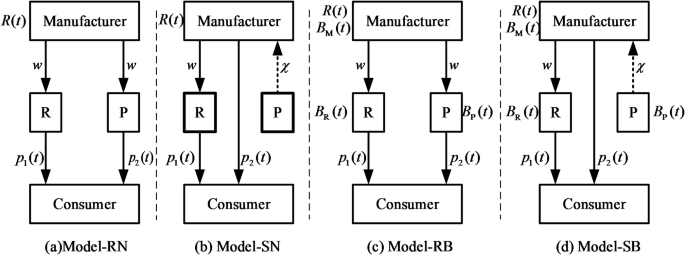
Pharmaceutical supply chain structure.
Reselling mode without blockchain (model RN)
In this scenario, both the e-commerce platform and traditional retailer purchase pharmaceuticals from the manufacturer at the same wholesale price, and independently determine retail prices. The manufacturer, traditional retailer, and e-commerce platform each aim to maximize their own profits, engaging in a Stackelberg differential game. The manufacturer first determines the wholesale price of the pharmaceutical, denoted as w. To guarantee the pharmaceutical quality, the manufacturer also determines the level of quality assurance inputs \(R(t)\). Subsequently, the traditional retailer and the e-commerce platform set their respective retail prices. The scenario is shown in Fig. 1a. Therefore, the differential game model for the three players is as follows:
$$\begin{gathered} J_{{\text{M}}}^{{{\text{RN}}}}=\mathop {\hbox{max} }\limits_{{{\text{R(t)}}}} \int_{0}^{{+\infty }} {{e^{ – \rho t}}} \left\{ {w\left[ {a – bp_{1}^{{{\text{RN}}}} – p_{2}^{{{\text{RN}}}}+\phi (p_{1}^{{{\text{RN}}}}+p_{2}^{{{\text{RN}}}}) – 2(1 – \Delta +h)\tau } \right]\theta {G^{{\text{RN}}}}\left( t \right) – \frac{1}{2}\kappa {{({R^{{\text{RN}}}})}^2}(t)} \right\}{\text{d}}t \hfill \\ J_{{\text{R}}}^{{{\text{RN}}}}=\mathop {\hbox{max} }\limits_{{p_{1}^{{{\text{RN}}}}(t)}} \int_{0}^{{+\infty }} {{e^{ – \rho t}}} \left\{ {(p_{1}^{{{\text{RN}}}} – w)\left[ {(1 – \eta )a – bp_{1}^{{{\text{RN}}}}+\phi p_{2}^{{{\text{RN}}}} – (1 – \Delta +h)\tau } \right]\theta {G^{{\text{RN}}}}(t)} \right\}{\text{d}}t \hfill \\ J_{{\text{P}}}^{{{\text{RN}}}}=\mathop {\hbox{max} }\limits_{{p_{2}^{{{\text{RN}}}}(t)}} \int_{0}^{{+\infty }} {{e^{ – \rho t}}} \left\{ {(p_{2}^{{{\text{RN}}}} – w)\left[ {\eta a – p_{2}^{{{\text{RN}}}}+\phi p_{1}^{{{\text{RN}}}} – (1 – \Delta +h)\tau } \right]\theta {G^{{\text{RN}}}}(t)} \right\}{\text{d}}t \hfill \\ s.t{{\dot {G}}^{{\text{RN}}}}(t)=\lambda {R^{{\text{RN}}}}(t) – \delta {G^{{\text{RN}}}}(t),G(0)={G_0} \hfill \\ \end{gathered}$$
(6)
In the above equation, \(J_{j}^{{{\text{RN}}}}(j=M,R,P)\) denotes the objective function of the supply chain members. The differential countermeasure model contains a state variable \(G(t)\) and a control variable \(R(t)\). By solving the optimal decision problem, the supply chain members can obtain optimal pricing and optimal quality assurance inputs to maximize the present value of profit over an infinite horizon (where the discount rate is \(\rho\)).
Proposition 1
The optimal equilibrium strategies for the manufacturer, traditional retailer and e-commerce platform in the RN scenario are
$$\begin{gathered} p_{1}^{{{\text{RN}}}}=\frac{{a[2(1 – \eta )+\eta \phi ] – 2wb – (\phi +2)(1 – \Delta +h)\tau +w\phi }}{{4b – {\phi ^2}}} \hfill \\ p_{2}^{{{\text{RN}}}}=\frac{{a[\phi (1 – \eta )+2b\eta ]+wb\phi – (\phi +2b)(1 – \Delta +h)\tau +2wb}}{{4b – {\phi ^2}}} \hfill \\ {R^{{\text{RN}}}}=\frac{{w[aM+N – L(1 – \Delta +h)\tau ]\theta \lambda }}{{\kappa S(\rho +\delta )}} \hfill \\ \end{gathered}$$
(7)
The temporal trajectory of pharmaceutical quality is \({G^{{\text{RN}}}}(t)=G_{0}^{{{\text{RN}}}}{e^{ – \delta t}}+G_{\infty }^{{{\text{RN}}}}(1 – {e^{ – \delta t}}){e^{ – \delta t}}\),\(G_{\infty }^{{{\text{RN}}}}=\frac{{w[aM+N – L(1 – \Delta +h)\tau ]\theta {\lambda ^2}}}{{\kappa \delta S(\rho +\delta )}}\) is the quality of the pharmaceutical at steady state, where\(M=\phi – \eta \phi +2b+b\eta \phi\),\(N=w[{b^2}+b{\phi ^2} – 2b+{\left( {b – \phi } \right)^2}]\),\(L=b\phi +4b+\phi\),\(S=(4b – {\phi ^2})\).
The profit function for the manufacturer, traditional retailer and e-commerce platform are\(V_{{\text{M}}}^{{{\text{RN}}}}={f_1}{G^{{\text{RN}}}}+{g_1},V_{{\text{R}}}^{{{\text{RN}}}}={f_2}{G^{{\text{RN}}}}+{g_2},V_{{\text{P}}}^{{{\text{RN}}}}={f_3}{G^{{\text{RN}}}}+{g_3}\). The values of \({f_i},{g_i}(i=1,2,3)\) and the proof procedure are shown in Supplementary Solution Process S1.
Proposition 1 states that all optimal strategies remain unchanged over time. It is evident that these decision variables are relatively static. However, the cost parameter, decay rate and discount factor negatively effect the decision variables of supply chain member. In this model, the pharmaceutical manufacturer can enhance quality assurance investments to improve pharmaceutical quality, thereby expanding demand and increasing profit.
Agency selling mode without blockchain (model SN)
In this scenario, the pharmaceutical manufacturer provides pharmaceuticals to traditional retailers at a fixed wholesale price, while the manufacturer enters the online channel, handling online sales of the pharmaceutical and paying a predefined commission rate to the platform. In this case, the e-commerce platform does not participate in the game. This situation is illustrated in Fig. 1b. Therefore, the differential game model between the manufacturer and the traditional retailer is as follows:
$$\begin{aligned} &J_{{\text{M}}}^{{{\text{SN}}}}=\mathop {\hbox{max} }\limits_{{{\text{R}}\left( t \right),p_{2}^{{{\text{SN}}}}}} \int_{0}^{{+\infty }} {{e^{ – \rho t}}}\nonumber\\ &\times\left\{ \begin{gathered} (1 – \chi )p_{2}^{{{\text{SN}}}}[\eta a – p_{2}^{{{\text{SN}}}}+\phi p_{1}^{{{\text{SN}}}} – (1 – \Delta +h)\tau ]\theta {G^{{\text{SN}}}}(t)+w[(1 – \eta )a – bp_{1}^{{{\text{SN}}}}+\phi p_{2}^{{{\text{SN}}}} – (1 – \Delta +h)\tau ]\theta {G^{{\text{SN}}}}(t) \hfill \\ – \frac{1}{2}\kappa {({R^{{\text{SN}}}})^2}(t) \hfill \\ \end{gathered} \right\}{\text{d}}t \nonumber\\ & J_{{\text{R}}}^{{{\text{SN}}}}=\mathop {\hbox{max} }\limits_{{p_{1}^{{{\text{SN}}}}}} \int_{0}^{{+\infty }} {{e^{ – \rho t}}} \left\{ {(p_{1}^{{{\text{SN}}}} – w)[(1 – \eta )a – bp_{1}^{{{\text{SN}}}}+\phi p_{2}^{{{\text{SN}}}} – (1 – \Delta +h)\tau ]\theta {G^{{\text{SN}}}}(t)} \right\}{\text{d}}t \nonumber\\ & s.t{{\dot {G}}^{{\text{SN}}}}(t)=\lambda {R^{{\text{SN}}}}(t) – \delta {G^{{\text{SN}}}}(t),G(0)={G_0} \end{aligned}$$
(8)
Proposition 2
The optimal equilibrium strategies of the traditional retailer, manufacturer under the SN model are
$$\begin{gathered} p_{1}^{{{\text{SN}}}}=\frac{{(1 – \chi )[a[2(1 – \eta )+\eta \phi ]+2wb – (\phi +2)(1 – \Delta +h)\tau ]+w{\phi ^2}}}{{(4b – {\phi ^2})(1 – \chi )}} \hfill \\ p_{2}^{{{\text{SN}}}}=\frac{{(1 – \chi )[a[\phi (1 – \eta )+2b\eta ]+wb\phi – (\phi +2b)(1 – \Delta +h)\tau ]+2wb\phi }}{{(4b – {\phi ^2})(1 – \chi )}} \hfill \\ {R^{{\text{SN}}}}=\frac{{[(X+2wb\phi )(X+Z\phi )+wY]\theta \lambda }}{{\kappa {S^2}(1 – \chi )(\rho +\delta )}} \hfill \\ \end{gathered}$$
(9)
The mass of the pharmaceutical is\({G^{{\text{SN}}}}(t)=G_{0}^{{{\text{SN}}}}{e^{ – \delta t}}+G_{\infty }^{{{\text{SN}}}}(1 – {e^{ – \delta t}})\), \(G_{\infty }^{{{\text{SN}}}}=\frac{{[(X+2wb\phi )(X+Z\phi )+wY]\theta {\lambda ^2}}}{{\kappa \delta {S^2}(1 – \chi )(\rho +\delta )}}\), where\(X=(1 – \chi )[a[\phi (1 – \eta )+2b\eta ]+wb\phi – (\phi +2b)(1 – \Delta +h)\tau ],\) \(Y=b[(1 – \chi )[a[2(1 – \eta )+\eta \phi ]+w({\phi ^2} – 2b) – (\phi +2)(1 – \Delta +h)\tau ]+w{\phi ^2}],\) \(Z=w({\phi ^2} – 2b)\).
The profit function for the manufacturer and the traditional retailer are \(V_{{\text{M}}}^{{{\text{SN}}}}={f_4}{G^{{\text{SN}}}}+{g_4}\),\(V_{{\text{R}}}^{{{\text{SN}}}}={f_5}{G^{{\text{SN}}}}+{g_5}\) respectively. The values of \({f_i},{g_i}(i=4,5)\) and the proof procedure are shown in Supplementary Solution Process S1.
Proposition 2 indicates that in the agency selling model, the reduction of intermediate steps in pharmaceutical sales allows the manufacturer, who holds the pricing power, to attract consumers by lowering the retail price in the online channel. This strategy not only increases online demand but also promotes higher profitability. At the same time, the manufacturer should invest more in quality assurance to improve the pharmaceutical quality. Additionally, the e-commerce platform should reasonably set the commission rate to attract manufacturers to join the platform, fostering a cooperative relationship that promotes product and market development, achieving a win-win situation.
Blockchain enabled reselling mode (model RB)
The scenario is similar to the scenario RN, but the difference is that, in this model, all supply chain members can meet consumers’ demands for pharmaceutical traceability. By introducing blockchain technology, end-to-end traceability of the pharmaceutical supply chain becomes a reality, enhancing transparency across the supply chain and increasing consumer trust in pharmaceuticals. The scenario is shown in Fig. 1(c). The corresponding differential game model for the three players is as follows:
$$\begin{gathered} J_{{\text{M}}}^{{{\text{RB}}}}=\mathop {\hbox{max} }\limits_{{{\text{R(t)}},{B_M}(t)}} \int_{0}^{{+\infty }} {{e^{ – \rho t}}} \left\{ {w[\varepsilon – bp_{1}^{{{\text{RB}}}} – p_{2}^{{{\text{RB}}}}+\phi (p_{1}^{{{\text{RB}}}}+p_{2}^{{{\text{RB}}}}) – 2\tau \bar {h}][\theta {G^{{\text{RB}}}}(t)+\beta {Q^{{\text{RB}}}}(t)] – \frac{1}{2}\kappa {{({R^{{\text{RB}}}})}^2}(t) – \frac{1}{2}{\mu _1}{{(B_{{\text{M}}}^{{{\text{RB}}}})}^2}(t)} \right\}{\text{d}}t \hfill \\ J_{{\text{R}}}^{{{\text{RB}}}}=\mathop {\hbox{max} }\limits_{{p_{1}^{{{\text{RB}}}}(t),{B_R}(t)}} \int_{0}^{{+\infty }} {{e^{ – \rho t}}} \left\{ {(p_{1}^{{{\text{RB}}}} – w)[(1 – \eta )\varepsilon – bp_{1}^{{{\text{RB}}}}+\phi p_{2}^{{{\text{RB}}}} – \tau \bar {h}][\theta {G^{{\text{RB}}}}(t)+\beta {Q^{{\text{RB}}}}(t)] – \frac{1}{2}{\mu _2}{{(B_{{\text{R}}}^{{{\text{RB}}}})}^2}(t)} \right\}{\text{d}}t \hfill \\ J_{{\text{P}}}^{{{\text{RB}}}}=\mathop {\hbox{max} }\limits_{{p_{2}^{{{\text{RB}}}}(t),{B_P}(t)}} \int_{0}^{{+\infty }} {{e^{ – \rho t}}} \left\{ {(p_{2}^{{{\text{RB}}}} – w)[\eta \varepsilon – p_{2}^{{{\text{RB}}}}+\phi p_{1}^{{{\text{RB}}}} – \tau \bar {h}][\theta {G^{{\text{RB}}}}(t)+\beta {Q^{{\text{RB}}}}(t)] – \frac{1}{2}{\mu _3}{{(B_{{\text{P}}}^{{{\text{RB}}}})}^2}(t)} \right\}{\text{d}}t \hfill \\ s.t\left\{ \begin{gathered} {{\dot {G}}^{{\text{RB}}}}(t)=\lambda {R^{{\text{RB}}}}(t) – \delta {G^{{\text{RB}}}}(t),G\left( 0 \right)={G_0} \hfill \\ {{\dot {Q}}^{{\text{RB}}}}(t)=\varphi B_{{\text{M}}}^{{{\text{RB}}}}(t)+\psi B_{{\text{R}}}^{{{\text{RB}}}}(t)+\omega B_{{\text{P}}}^{{{\text{RB}}}}(t) – \alpha {Q^{{\text{RB}}}}(t),Q(0)={Q_0} \hfill \\ \end{gathered} \right. \hfill \\ \end{gathered}$$
(10)
Proposition 3
Under the RB model, the optimal equilibrium strategies for the manufacturer, traditional retailer and e-commerce platform are
$$\begin{gathered} p_{1}^{{{\text{RB}}}}=\frac{{\varepsilon [2(1 – \eta )+\eta \phi ] – 2wb – (\phi +2)\tau \bar {h}+w\phi }}{{4b – {\phi ^2}}} \hfill \\ p_{2}^{{{\text{RB}}}}=\frac{{\varepsilon [\phi (1 – \eta )+2b\eta ]+wb\phi – (\phi +2b)\tau \bar {h}+2wb}}{{4b – {\phi ^2}}} \hfill \\ {R^{{\text{RB}}}}=\frac{{w(\varepsilon M+N – L\tau \bar {h})\theta \lambda }}{{\kappa S(\rho +\delta )}} \hfill \\ B_{{\text{M}}}^{{{\text{RB}}}}=\frac{{w(\varepsilon M+N – L\tau \bar {h})\beta \varphi }}{{{\mu _1}S(\rho +\alpha )}} \hfill \\ B_{{\text{R}}}^{{{\text{RB}}}}=\frac{{b(E – 6wb)(E+2wb)\beta \psi }}{{{\mu _2}{S^2}(\rho +\alpha )}} \hfill \\ B_{{\text{P}}}^{{{\text{RB}}}}=\frac{{(F+wb\phi )(F – 3wb\phi )\beta \omega }}{{{\mu _3}{S^2}(\rho +\alpha )}} \hfill \\ \end{gathered}$$
(11)
The mass of the pharmaceutical is\({G^{{\text{RB}}}}(t)=G_{0}^{{{\text{RB}}}}{e^{ – \delta t}}+G_{\infty }^{{{\text{RB}}}}(1 – {e^{ – \delta t}})\), \(G_{\infty }^{{{\text{RB}}}}=\frac{{w(\varepsilon M+N – L\tau \bar {h})\theta {\lambda ^2}}}{{\kappa \delta S(\rho +\delta )}}\).
The level of blockchain-enabled pharmaceutical traceability is\({Q^{{\text{RB}}}}(t)=Q_{0}^{{{\text{RB}}}}{e^{ – \alpha t}}+Q_{\infty }^{{{\text{RB}}}}(1 – {e^{ – \alpha t}})\), \(Q_{\infty }^{{{\text{RB}}}}=\frac{{w(\varepsilon M+N – L\tau \bar {h})\beta {\varphi ^2}}}{{{\mu _1}\alpha S(\rho +\alpha )}}+\frac{{b(E – 6wb)(E+2wb)\beta {\psi ^2}}}{{{\mu _2}\alpha {S^2}(\rho +\alpha )}}+\frac{{(F+wb\phi )(F – 3wb\phi )\beta {\omega ^2}}}{{{\mu _3}\alpha {S^2}(\rho +\alpha )}}\) indicates the level of pharmaceutical traceability at steady state, where\(E=\varepsilon [2(1 – \eta )+\eta \phi ]+w(\phi +{\phi ^2}) – (\phi +2)\tau \bar {h}\), \(F=\varepsilon [\phi (1 – \eta )+2b\eta ]+w({\phi ^2} – 2b) – (\phi +2b)\tau \bar {h}\).
The profit function for the manufacturer, traditional retailer and e-commerce platform are\(V_{{\text{M}}}^{{{\text{RB}}}}={f_6}{G^{{\text{RB}}}}+{h_6}{Q^{{\text{RB}}}}+{g_6}\),\(V_{{\text{R}}}^{{{\text{RB}}}}={f_7}{G^{{\text{RB}}}}+{h_7}{Q^{{\text{RB}}}}+{g_7}\),\(V_{{\text{P}}}^{{{\text{RB}}}}={f_8}{G^{{\text{RB}}}}+{h_8}{Q^{{\text{RB}}}}+{g_8}\). The values of \({f_i},{h_i},{g_i}(i=6,7,8)\) and the proof procedure are shown in Supplementary Solution Process S1.
Proposition 3 suggests that as the larger the market size increases, the greater the potential for profit and the opportunity for profit growth. Supply chain members are more motivated to invest in pharmaceutical quality and traceability. Furthermore, as the proportion of online shopping increases, e-commerce platforms are increasingly enthusiastic about technology investment. Rising costs will drive platforms to raise the retail prices for online channels, but consumers’ preference for online channels will reduce their price sensitivity, increasing online demand and improving profitability.
Blockchain enabled agency selling mode (model SB)
This scenario builds upon Scenario SN but incorporates blockchain technology. With the introduction of blockchain by the manufacturer, traditional retailer and e-commerce platform, all production information can be recorded on a blockchain platform like Ethereum. All supply chain members and consumers can access the relevant information through an app. The scenario is depicted in Fig. 1(d). Therefore, the differential game model of the three parties is as follows:
$$\begin{gathered} J_{{\text{M}}}^{{{\text{SB}}}}=\mathop {\hbox{max} }\limits_{{{\text{R}}\left( t \right),{B_{\text{M}}}{\text{(}}t),p_{2}^{{{\text{SN}}}},}} \int_{0}^{{+\infty }} {{e^{ – \rho t}}} \left\{ \begin{gathered} (1 – \chi )p_{2}^{{{\text{SB}}}}[\eta \varepsilon – p_{2}^{{{\text{SB}}}}+\phi p_{1}^{{{\text{SB}}}} – \tau \bar {h}][\theta {G^{{\text{SB}}}}(t)+\beta {Q^{{\text{SB}}}}(t)] \hfill \\ +w[(1 – \eta )\varepsilon – bp_{1}^{{{\text{SB}}}}+\phi p_{2}^{{{\text{SB}}}} – \tau \bar {h}][\theta {G^{{\text{SB}}}}(t)+\beta {Q^{{\text{SB}}}}(t)] – \frac{1}{2}\kappa {({R^{{\text{SB}}}})^2}(t) – \frac{1}{2}{\mu _1}{(B_{{\text{M}}}^{{{\text{SB}}}})^2}(t) \hfill \\ \end{gathered} \right\}{\text{d}}t \hfill \\ J_{{\text{R}}}^{{{\text{SB}}}}=\mathop {\hbox{max} }\limits_{{p_{1}^{{{\text{SB}}}},{B_{\text{R}}}{\text{(}}t)}} \int_{0}^{{+\infty }} {{e^{ – \rho t}}} \left\{ {(p_{1}^{{{\text{SB}}}} – w)[(1 – \eta )\varepsilon – bp_{1}^{{{\text{SB}}}}+\phi p_{2}^{{{\text{SB}}}} – \tau \bar {h}][\theta {G^{{\text{SB}}}}(t)+\beta {Q^{{\text{SB}}}}(t)] – \frac{1}{2}{\mu _2}{{(B_{{\text{R}}}^{{{\text{SB}}}})}^2}(t)} \right\}{\text{d}}t \hfill \\ J_{{\text{P}}}^{{{\text{SB}}}}=\mathop {\hbox{max} }\limits_{{{B_{\text{P}}}\left( t \right)}} \int_{0}^{{+\infty }} {{e^{ – \rho t}}} \left\{ {\chi p_{2}^{{{\text{SB}}}}[\eta \varepsilon – p_{2}^{{{\text{SB}}}}+\phi p_{1}^{{{\text{SB}}}} – \tau \bar {h}][\theta {G^{{\text{SB}}}}(t)+\beta {Q^{{\text{SB}}}}(t)] – \frac{1}{2}{\mu _3}{{(B_{{\text{P}}}^{{{\text{SB}}}})}^2}(t)} \right\}{\text{d}}t \hfill \\ s.t\left\{ \begin{gathered} {{\dot {G}}^{{\text{SB}}}}\left( t \right)=\lambda {R^{{\text{SB}}}}\left( t \right) – \delta {G^{{\text{SB}}}}\left( t \right),G\left( 0 \right)={G_0} \hfill \\ {{\dot {Q}}^{{\text{SB}}}}\left( t \right)=\varphi B_{{\text{M}}}^{{{\text{SB}}}}\left( t \right)+\psi B_{{\text{R}}}^{{{\text{SB}}}}\left( t \right)+\omega B_{{\text{P}}}^{{{\text{SB}}}}\left( t \right) – \alpha {Q^{{\text{SB}}}}\left( t \right),Q\left( 0 \right)={Q_0} \hfill \\ \end{gathered} \right. \hfill \\ \end{gathered}$$
(12)
Proposition 4
Under the SB model, the optimal equilibrium strategies of the manufacturer, traditional retailer and e-commerce platform are
$$\begin{gathered} p_{1}^{{{\text{SB}}}}=\frac{{(1 – \chi )[\varepsilon [2(1 – \eta )+\eta \phi ]+2wb – (\phi +2)\tau \bar {h}]+w{\phi ^2}}}{{(4b – {\phi ^2})(1 – \chi )}} \hfill \\ p_{2}^{{{\text{SB}}}}=\frac{{(1 – \chi )[\varepsilon [\phi (1 – \eta )+2b\eta ]+wb\phi – (\phi +2b)\tau \bar {h}]+2wb\phi }}{{(4b – {\phi ^2})(1 – \chi )}} \hfill \\ {R^{{\text{SB}}}}=\frac{{[(V+2wb\phi )(V+Z\phi )+wU]\theta \lambda }}{{\kappa {S^2}(1 – \chi )(\rho +\delta )}} \hfill \\ B_{{\text{M}}}^{{{\text{SB}}}}=\frac{{[(V+2wb\phi )(V+Z\phi )+wU]\beta \varphi }}{{{\mu _1}{S^2}(1 – \chi )(\rho +\delta )}} \hfill \\ B_{{\text{R}}}^{{{\text{SB}}}}=\frac{{\left\{ {(1 – \chi )[\varepsilon [2(1 – \eta )+\eta \phi ] – 2wb – (\phi +2)\tau \bar {h}]+2w{\phi ^2}} \right\}U\beta \psi }}{{{\mu _2}{S^2}{{(1 – \chi )}^2}(\rho +\alpha )}} \hfill \\ B_{{\text{P}}}^{{{\text{SB}}}}=\frac{{\chi (V+2wb\phi )(V+Z\phi )\beta \omega }}{{{\mu _3}S(1 – \chi )(\rho +\alpha )}} \hfill \\ \end{gathered}$$
(13)
The mass of the pharmaceutical is \({G^{{\text{SB}}}}(t)=G_{0}^{{{\text{SB}}}}{e^{ – \delta t}}+G_{\infty }^{{{\text{SB}}}}(1 – {e^{ – \delta t}})\), \(G_{\infty }^{{{\text{SB}}}}=\frac{{\left[ {(V+2wb\phi )(V+Z\phi )+wU} \right]\theta {\lambda ^2}}}{{\kappa \delta {S^2}(1 – \chi )(\rho +\delta )}}\).
The level of blockchain-enabled pharmaceutical traceability is \({Q^{{\text{SB}}}}(t)=Q_{0}^{{{\text{SB}}}}{e^{ – \alpha t}}+Q_{\infty }^{{{\text{SB}}}}(1 – {e^{ – \alpha t}})\), \(Q_{\infty }^{{{\text{SB}}}}=\frac{{[(V+2wb\phi )(V+Z\phi )+wU]\beta {\varphi ^2}}}{{{\mu _1}\alpha {S^2}(1 – \chi )(\rho +\delta )}}+\frac{{\left\{ {(1 – \chi )[\varepsilon [2(1 – \eta )+\eta \phi ] – 2wb – (\phi +2)\tau \bar {h}]+2w{\phi ^2}} \right\}U\beta {\psi ^2}}}{{{\mu _2}\alpha {S^2}{{(1 – \chi )}^2}(\rho +\alpha )}}+\frac{{\chi (V+2wb\phi )(V+Z\phi )\beta {\omega ^2}}}{{{\mu _3}\alpha S(1 – \chi )(\rho +\alpha )}}\), where\(U=b\left\{ {(1 – \chi )[\varepsilon [2(1 – \eta )+\eta \phi ] – 2wb – (\phi +2)\tau \bar {h}]+2w{\phi ^2}} \right\}\), \(V=(1 – \chi )[\varepsilon [\phi (1 – \eta )+2b\eta ]+wb\phi – (\phi +2b)\tau \bar {h}]\).
The profit function for the manufacturer, traditional retailer, and e-commerce platform are, \(V_{{\text{M}}}^{{{\text{SB}}}}={f_9}{G^{{\text{SB}}}}+{h_9}{Q^{{\text{SB}}}}+{g_9}\), \(V_{{\text{R}}}^{{{\text{SB}}}}={f_{10}}{G^{{\text{SB}}}}+{h_{10}}{Q^{{\text{SB}}}}+{g_{10}}\),\(V_{{\text{P}}}^{{{\text{SB}}}}={f_{11}}{G^{{\text{SB}}}}+{h_{11}}{Q^{{\text{SB}}}}+{g_{11}}\). The values of \({f_i},{h_i},{g_i}(i=9,10,11)\) and the proof procedure are shown in Supplementary Solution Process S1.
Proposition 4 indicates that the pharmaceutical retail price will rise following the introduction of blockchain technology, in contrast to the scenario where blockchain without it. However, the transparency of the sales process not only enhances the traceability of the supply chain, ensuring the safety performance of the pharmaceuticals purchased by consumers, but also builds consumer trust, making them more willing to pay premium prices for pharmaceuticals. As a result, market demand for pharmaceuticals expands, leading to higher profitability for supply chain members. The pharmaceutical manufacturer is also more inclined to increase its investment in pharmaceutical quality assurance. Moreover, in the long term, the introduction of blockchain technology will further promote the development of enterprises.
link


